Discrete Calculus for DeFi Math

Hello everyone and welcome to the CavalRe! 🤠

In this article, I present a primer on discrete calculus with the intention of helping us analyze DeFi protocols running on blockchains, which are inherently discrete in nature.

Blockchain as a State Machine

The Ethereum yellow paper describes the Ethereum blockchain as a state machine with the state of the world denoted by $\sigma(t)$. Given a transaction $T(t,t+1)$, the state is updated to a new state $\sigma(t+1)$ by the Ethereum state transition function $\Upsilon$ denoted by

$$\sigma(t+1) = \Upsilon(\sigma(t),T(t,t+1)).$$

It is important to note the inherent discreteness of this process. There is no state between $\sigma(t)$ and $\sigma(t+1).$ A transaction takes you from some initial state to some final state with nothing in between and repeats indefinitely with every new transaction.

This discreteness has implications for how we should analyze blockchain protocols such as automated market makers (AMMs) so we will enhance our toolbox for dealing with this discreteness in the remainder of this article.

Node Functions

Every blockchain needs to start with some initial state created by some kind of genesis event. Therefore, it makes sense to restrict $t$ to be a natural number $\N$ with the initial state denoted $\sigma_0.$ A node function is simply a function

$$f: \N\to\R,$$

where $\R$ denotes real numbers. Let $\mathbf{e}^t$ denote a special function whose value is given by

$$\mathbf{e}^t(t') = \begin{cases} 1 &\text{if } t = t',\\ 0 &\text{otherwise.} \end{cases}$$

Any node function $f:\N\to\R$ can be expressed as a linear combination of these functions, i.e.

$$f = \sum_{t\in\N} f(t) \mathbf{e}^t,$$

where $f(t)\in\R$ is the value of $f$ at $t$. The basis functions can be multiplied

$$\mathbf{e}^t \mathbf{e}^{t'} = \begin{cases} \mathbf{e}^t &\text{if } t = t',\\ 0 &\text{otherwise} \end{cases}$$

which extends to the product of arbitrary node functions $f,g:\N\to\R$ intuitively as

$$f g = \sum_{t\in\N} f(t) g(t) \mathbf{e}^t.$$

The product of two node functions is commutative, i.e. $f g = g f$, just like the product of continuous functions.

Edge Functions

The natural numbers $\N$ can be thought of as a simple directed graph. In the context of blockchain, the state $\sigma(t)$ would then reside on the node $t,$ whereas the transaction $T(t,t+1)$ would reside on the directed edge between states $\sigma(t)$ and $\sigma(t+1)$ as illustrated below.

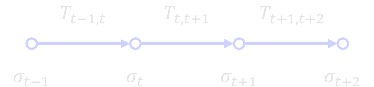
Letting $d\N$ denote the set of edges between natural numbers when thinking of $\N$ as a directed graph, define functions $\mathbf{e}^{t,t+1}: d\N\to\R$ by

$$\mathbf{e}^{t,t+1}(t',t'+1) = \begin{cases} 1 &\text{if } t = t',\\ 0 &\text{otherwise.} \end{cases}$$

We can then define a general discrete edge function $T$ as a linear combination

$$T = \sum_{t\in\N} T(t,t+1) \mathbf{e}^{t,t+1},$$

where $T(t,t+1)$ is the value of $T$ on the edge $(t,t+1).$

Multiplication of an edge function by a node function on the left can be defined in terms of basis functions via

$$\mathbf{e}^t \mathbf{e}^{t',t'+1} = \begin{cases} e^{t,t+1} &\text{if } t = t',\\ 0 &\text{otherwise.} \end{cases}$$

In other words, the product is zero unless the node coincides with the beginning of the edge. Similarly, multiplication of an edge function by a node function on the right can be defined in terms of basis functions via

$$\mathbf{e}^{t,t+1} \mathbf{e}^{t'} = \begin{cases} e^{t,t+1} &\text{if } t+1 = t',\\ 0 &\text{otherwise.} \end{cases}$$

In other words, the product is zero unless the node coincides with the end of the edge. In general we have

$$f T = \sum_{t\in\N} f(t) T(t,t+1) \mathbf{e}^{t,t+1}$$

and

$$T f = \sum_{t\in\N} f(t+1) T(t,t+1) \mathbf{e}^{t,t+1}$$

so that the product of node functions and edge functions is noncommutative, i.e. $f T \neq T f.$

There is also a natural product of edge functions defined by

$$\mathbf{e}^{t,t+1}\bullet \mathbf{e}^{t',t'+1} = \begin{cases} e^{t,t+1} &\text{if } t = t',\\ 0 &\text{otherwise.} \end{cases}$$

so that

$$U\bullet V = \sum_{t\in\N} U(t,t+1)V(t,t+1) e^{t,t+1}$$

and the product of edge functions is commutative, i.e. $U\bullet V = V\bullet U$.

Discrete Differentials

There is a special "unit" node function

$$1 = \sum_{t\in\N} \mathbf{e}^t$$

that satisfies $1 f = f 1 = f$ and $1 T = T 1 = T.$ Similarly, there is a special "graph" edge function

$$G = \sum_{t\in\N} \mathbf{e}^{t,t+1}$$

that acts as an identity on other edge functions, i.e.

$$T\bullet G = G\bullet T = T.$$

With the graph edge function, we can define the differential of a node function $f$ via

$$d f = [G,f],$$

where $[G,f] = G f - f G$ denotes the commutator, i.e.

$$d f = \sum_{t\in\N} \Delta f(t,t+1) \mathbf{e}^{t,t+1}$$

with

$$\Delta f(t,t+1) = f(t+1) - f(t).$$

It follows from the properties of the commutator that

$$[G,f g] = [G,f] g + f [G,g]$$

which gives rise to the discrete product rule

$$d(f g) = (d f) g + f (d g).$$

Although the product of node functions on the left-hand side is commutative, the products on the right-hand side are noncommutative so the order they are written matters. The above can be expressed in terms of the commutative product of edge functions via

$$d(f g) = d f\bullet G g + f G\bullet d g.$$

We could have also written the discrete product rule as

$$d(g f) = (d g) f + g (d f).$$

or

$$d(g f) = d g\bullet G f + g G\bullet d f.$$

This means that when dealing with discrete node and edge functions, as we must with blockchain protocols, we have a degree of freedom in how we decompose terms in the discrete product rule since we can take linear combinations of the above two expressions and the result is a valid expression:

$$\begin{align*} d(f g) &= df\bullet\left[k G g + (1-k) g G\right] + \left[k f G + (1-k) G f\right]\bullet dg \end{align*}$$

Let us introduce the notation

$$E_k f = (1-k) f G + k G f$$

so that the general discrete product rule can be written as

$$d(f g) = df\bullet E_k g + E_{1-k} f\bullet d g.$$

Case: $k=0$

$$\Delta(f g)(t,t+1) = \Delta f(t,t+1) g(t) + f(t+1) \Delta g(t,t+1)$$

Case: $k=1/2$

$$\Delta(f g)(t,t+1) = \Delta f(t,t+1) \frac{g(t)+g(t+1)}2 + \frac{f(t)+f(t+1)}2 \Delta g(t,t+1)$$

Case: $k=1$

$$\Delta(f g)(t,t+1) = \Delta f(t,t+1) g(t+1) + f(t) \Delta g(t,t+1)$$

The value of $k$ has no impact on the sum. It merely impacts the way the discrete product rule decomposes into the two terms. As we will see in subsequent articles, this degree of freedom stemming from the inherent discreteness of a blockchain has important implications for AMM design.

Closer look 🧐: Note on Symmetries

There is a symmetry given by

$$E_k f(t,t+1) = E_{1-k} f(t+1,t)$$

and

$$\Delta f(t,t+1) = -\Delta f(t+1,t).$$

In other words, if the direction of time is reversed so that $t$ and $t+1$ are swapped, then we can simply replace $k$ with $1-k$ in the discrete product rule. This means that:

• The discrete product rule for $k=0$ is equivalent to the discrete product rule for $k=1$ with time reversed;
• The discrete product rule for $k=1$ is equivalent to the discrete product rule for $k=0$ with time reversed; and
• The discrete product rule for $k=1/2$ is the same whether forward in time or time reversed.

We will see this again when looking at self-financing in DeFi protocols.